YOLOv7: Training bag-of-freebies sets new state-of-the-art for real-time object detectors
This paper ficus on some optimized modules and optimization methods which may strengthen the training cost for improving the accuracy of object detection, but without increasing the inference cost. The proposed modules and optimization methods are called trainable bag-of-freebies.
Two improved architecture (E-ELAN and model scaling for concatenation-based models) and two trainable bag-of-freebies (planned re-parameterized convolution, coarse for auxiliary and fine for lead loss) are proposed in this paper.
Architecture
Proposed architecture: E-ELAN
The main considerations are no more than the number of parameters, the amount of computation, and the computational density.
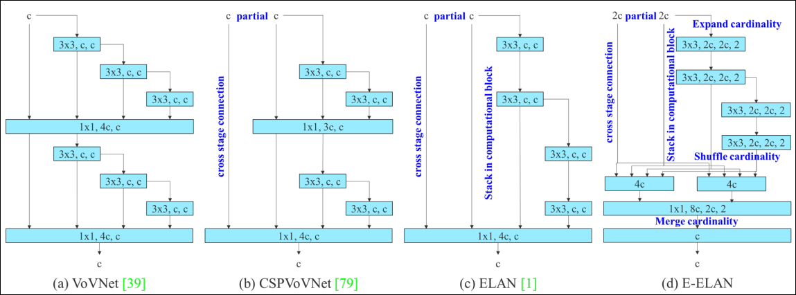
CSP VoVNet
The design of CSPVoVNet in sub-figure(b) is a variation of VoVNet, shown in sub-figure (a). In addition to considering the aforementioned basic designing concerns, the architecture of CSPVoVNet also analyzes the gradient path, in order to enable the weights of different layers to learn more diverse features.
The gradient analysis approach described above makes inferences faster and more accurate.
ELAN
ELAN gives the conclusion: By controlling the shortest longest gradient path, a deeper network can learn and converge effectively.
E-ELAN
Extended-ELAN (E-ELAN) is based on ELAN and its main architecture, shown in sub-figure (d).
The stable state maybe destroyed if more computational blocks are stacked unlimitedly, and the parameter utilization rate will also decrease. To solve the problem, E-ELAN uses expand, shuffle, merge cardinality to achieve the ability to continuously enhance the learning ability of the network without destroying the original gradient path.
Change. only change the architecture in computational blocks, while the architecture of the transition layer is completely unchanged.
Strategy. Use group convolution to expand the channel and cardinality of computational blocks.
The feature map calculated by each computational block will be shuffled into $g$ groups according to the set group parameter $g$, and then concatenate them together.
At this time, the number of channels in each group of feature map will be the same as the number of channels in the original architecture.
Finally, we add $g$ groups of feature maps to perform merge cardinality.
In addition to maintaining the original ELAN design architecture, E-ELAN can also guide different groups of computational blocks to learn more diverse features.
Model scaling for concatenation-based models
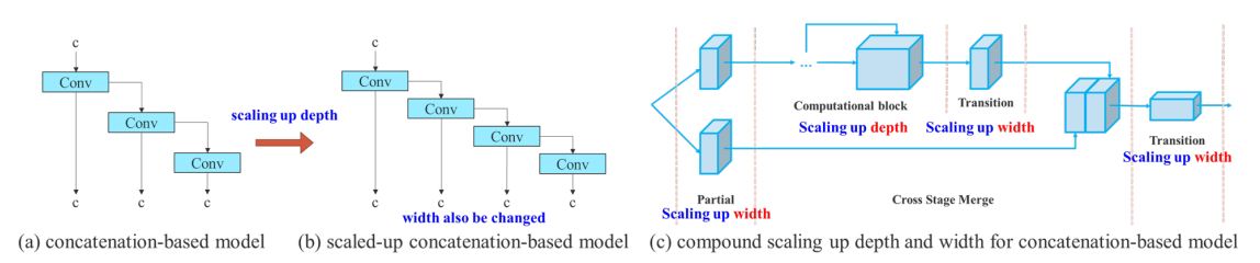
For concatenation-based architectures, scaling up or scaling down is performed on depth, the in-degree of a translation layer which is immediately after a concatenation-based computational block will decrease or increase, shown in sub-figure (a) and (b).
Take scaling-up depth as an example, such an action will cause a ratio change between the input channel and output channel of a transition layer, which may lead to a decrease in the hardware usage of the model. Therefore, we must propose the corresponding compound model scaling method for a concatenation-based model. When we scale the depth factor of a computational block, we must also calculate the change of the output channel of that block. Then, we will perform width factor scaling with the same amount of change on the transition layers, and the result is shown in sub-figure (c). Our proposed compound scaling method can maintain the properties that the model had at the initial design and maintains the optimal structure.
A transition layer is like one by one convolution followed by Max pooling to reduce the size of the feature maps. So the transition layer allows for Max pooling, which typically leads to a reduction in the size of your feature maps.
Trainable bag-of-freebies
Planned re-parameterized convolution
- Gradient flow propagation paths are used to analyze how re-parameterized convolution should be combined with different network.
- Planned re-parameterized convolution is also designed accordingly
RepConv without identity connection (RepConvN) are used to design the architecture of planned re-parameterized convolution.
RepConv actually combines 3 × 3 convolution, 1 × 1 convolution, and identity connection in one convolutional layer.
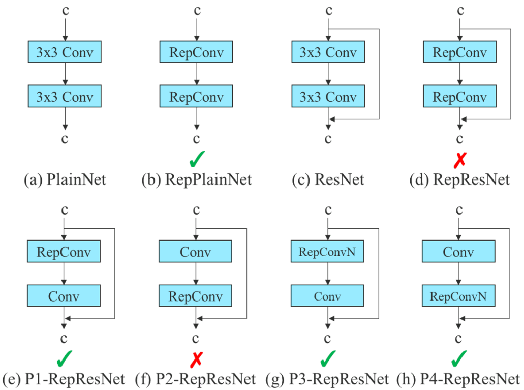
In the proposed planned re-parameterized model, we found that a layer with residual or concatenation connections, its RepConv should not have identity connection. Under these circumstances, it can be replaced by RepConvN that contains no identity connections.
Coarse for auxiliary and fine for lead loss

The head responsible for the final output as the lead head, and the head used to assist training is called auxiliary head.
Deep supervision is a technique that is often used in training deep networks. Its main concept is to add extra auxiliary head in the middle layers of the network, and the shallow network weights with assistant loss as the guide.
Label assigner refers to the mechanism that considers the network prediction results together with the ground truth and then assigns soft labels.
Lead head guided label assigner
Lead head guided label assigner is mainly calculated based on the prediction results of lead head and the ground truth, and generate soft labels through the optimization process.
This set of soft labels will be used as the target training model for both auxiliary head and lead head. The reason to do this is because lead head has a relatively strong learning capability, so the soft label generated from it should be more representative of the distribution and correlation between the source data and the target.
Coarse-to-fine lead head guided label assigner
Difference to the previous label assigner (Lead head guided label assigner) is the two different sets of soft label we generated in the process, i.e., coarse label and fine label, where fine label is the same as the soft label generated by lead head guided label assigner, and coarse labels generated by allowing more grids to be treated as positive target by relaxing the constraints of the positive sample assignment process.
Reason. The learning ability of an auxiliary head is not as strong as that of a lead head, and in order to avoid losing the information that needs to be learned, we will focus on optimizing the recall of auxiliary head in the object detection task.
- As for the output of lead head, we can filter the high precision results from the high recall results as the final output.
- In order to make those extra coarse positive grids have less impact, we put restrictions in the decoder, so that the extra coarse positive grids cannot produce soft label perfectly.
The mechanism mentioned above allows the importance of fine label and coarse label to be dynamically adjusted during the learning process, and makes the optimizable upper bound of fine label always higher than coarse label.
Related works
Real-time object detectors
Being able to become a state-of-the-art real-time object detector usually requires the following characteristics:
- a faster and stronger network architecture;
- a more effective feature integration method;
- a more accurate detection method;
- a more robust loss function;
- a more efficient label assignment method;
- and a more efficient training method.
This paper design new trainable bag-of-freebies methods for the issues derived from the state-of-the-art methods associated with (4), (5), and (6) mentioned above.
Model re-parameterization
Model re-parameterization techniques merge multiple computational modules into one at inference stage, which can be regarded as an ensemble techniques. It can be divided into TWO categories:
- module-level ensemble
- model-level ensemble
model-level
Two common practice of model-level re-parameterization:
- train multiple identical models with different training data, and then average the weights of multiple trained models.
- perform a weighted average of the weights of models at different iteration number.
module-level
The method of model-level re-parameterization splits a module into multiple identical or different module branches during training and integrates multiple branched modules into a completely equivalent module during inference.
Model scaling
Model scaling is a way to scale up or down an already designed model and make it fit in different computing devices.
Different scaling factors:
- resolution (size of input image)
- depth (number of layer)
- width (number of channel)
- stage (number of feature pyramid)
Network architecture search (NAS) is one of the most commonly used model scaling methods.
- Advantages: automatically search for suitable scaling factors from search space without defining too complicated rules.
- Disadvantages: requires very expensive computation to complete the search for model scaling factors.
Almost all model scaling methods analyze individual scaling factor independently, and even the methods in the compound scaling category also optimized scaling factor independently.
A new compound model scaling method are designed for concatenation-based models in this paper, which tries to process the width and depth concurrently.
Highway network
In machine learning, the Highway Network was the first working very deep feedforward neural network with hundreds of layers, much deeper than previous artificial neural networks. It uses skip connections modulated by learned gating mechanisms to regulate information flow, inspired by Long Short-Term Memory (LSTM) recurrent neural networks. The advantage of a Highway Network over the common deep neural networks is that it solves or partially prevents the vanishing gradient problem, thus leading to easier to optimize neural networks. The gating mechanisms facilitate information flow across many layers ("information highways").
Gating mechanisms are widely used in neural network models, where they allow gradients to back-propagate more easily through depth or time.
Residual neural network (ResNet)
A residual neural network (ResNet) is an artificial neural network (ANN). It is a gateless or open-gated variant of the HighwayNet, the first working very deep feedforward neural network with hundreds of layers, much deeper than previous neural networks.
Skip connections or shortcuts are used to jump over some layers (HighwayNets may also learn the skip weights themselves through an additional weight matrix for their gates).
Concatenation, summation and aggregation
- Concatenation generally consists of taking 2 or more output tensors from different network layers and concatenating them along the channel dimension
- Aggregation consists in taking 2 or more output tensors from different network layers and applying a chosen multivariate function on them to aggregate the results
- Summation is a special case of aggregation where the function is a sum
This implies that we lose information by doing aggregation. On the other hand, concatenation will make it possible to retain information at the cost of greater memory usage.
References
- Wang C Y, Bochkovskiy A, Liao H Y M. YOLOv7: Trainable bag-of-freebies sets new state-of-the-art for real-time object detectors[J]. arXiv preprint arXiv:2207.02696, 2022.
- https://www.analyticsvidhya.com/blog/2022/03/introduction-to-densenets-dense-cnn/
- https://en.wikipedia.org/wiki/Highway_network
- Gu A, Gulcehre C, Paine T, et al. Improving the gating mechanism of recurrent neural networks[C]//International Conference on Machine Learning. PMLR, 2020: 3800-3809.
- https://en.wikipedia.org/wiki/Residual_neural_network