MIT Introduction to Deep Learning | 6.S191

Published: December 02, 2021 by Authur Lee

• Categories:
• Youtube_courses 6

• Tags:
• Deep Learning 5
• MIT 5

If you wanna see the original video, click MIT Introduction to Deep Learning $\vert$ 6.S191.

Lecture 1: Foundations of Deep Learning

What's Deep Learning?

• Artificial Intelligence: Any technique that enables computers to mimic human behavior.
  • Machine Learning: Ability to learn without explicitly being programmed.
    • Deep Learning: Extract patterns from data using neural networks.

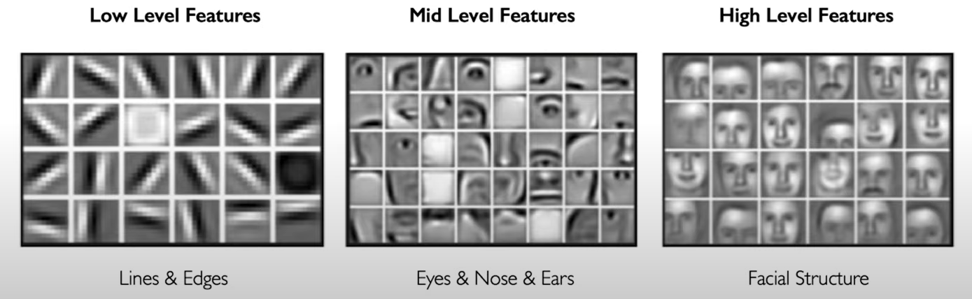
How is deep learning is different from traditional machine learning? Traditionally, machine learning algorithms define a set of features of the data, usually these are features that are handcrafted or hand engineered and as a result they tend to be pretty brittle in practice when they're deployed. The key idea of deep learning is to learn these features directly from data in a hierarchical manner that is can we learn if we want to learn. (the explanation of word "hierarchical" is below)

The Perceptron: The structural building block of deep learning

The perceptron: Forward Propagation.

\[\hat{y}=g(w_0+X^TW),\\~\\ \text{where: }X=\begin{bmatrix} x_1\\:\\ x_m \end{bmatrix}\text{and }W=\begin{bmatrix} w_1\\:\\ w_m \end{bmatrix}\]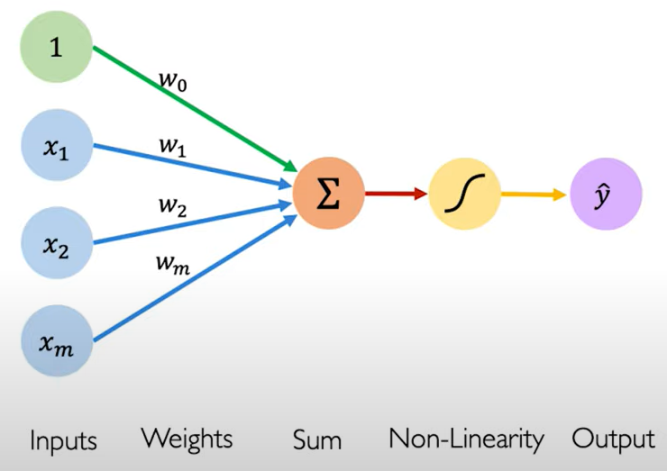

• $g$ is Non-Linearity, which one of its examples is a sigmoid function

TIPS. Pay attention to the figure above, and you will get more than you want.

\[g(z)=\sigma(z)=\frac{1}{1+e^z}\]

Common Activation Functions:

• Sigmoid Function: $g(z)=\frac{1}{1+e^z},~g'(z)=g(z)(1-g(z))$
• Hyperbolic Function: $g(z)=\frac{e^z-e^{-z}}{e^z+e^{-z}},~g'(z)=1-g(z)^2$
• Rectified Linear Unit (ReLU): $g(z)=max(0,z),~g'(z)=\text{I}{z>0}$

tf.math.sigmoid(z)
tf.math.tanh(z)
tf.nn.relu(z)

All activation functions are non-linear.

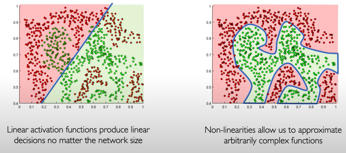
The purpose of activation functions. The purpose is to introduce non-linearities into the network.

in this world, the data is always non-linear.

Non-linearities allow us to approximate arbitrarily complex functions.

Building Neural Networks with Perceptrons

class MyDenseLayer(tf.keras.layers.Layer):
    def __init__(self, input_dim, output_dim):
        super(MyDenseLayer, self).__init__()

        # Initialize weights and bias
        self.W = self.add_weight([input_dim, output_dim])
        self.b = self.add_weight([1, output_dim])
    
    def call(self, inputs):
        # Forward propagate the inputs
        z = tf.matmul(inputs, self.W) + self.b

        # Feed through a non-linear activation
        output = tf.math.sigmoid(z)

        return output

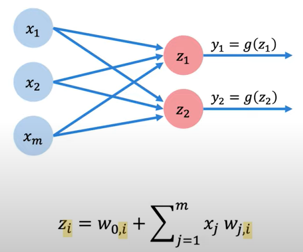
Multi Output Perceptron.

import tensorflow as tf

layer = tf.keras.layers.Dense(units=2)

Dense layers. Because all inputs are densely connected to all outputs, these layers are called Dense layers.

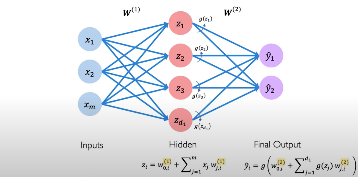
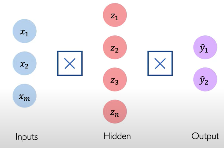
Single Layer Neural Network.

import tensorflow as tf

model = tf.keras.Sequential([
    tf.keras.layers.Dense(n),
    tf.keras.layers.Dense(2)
])

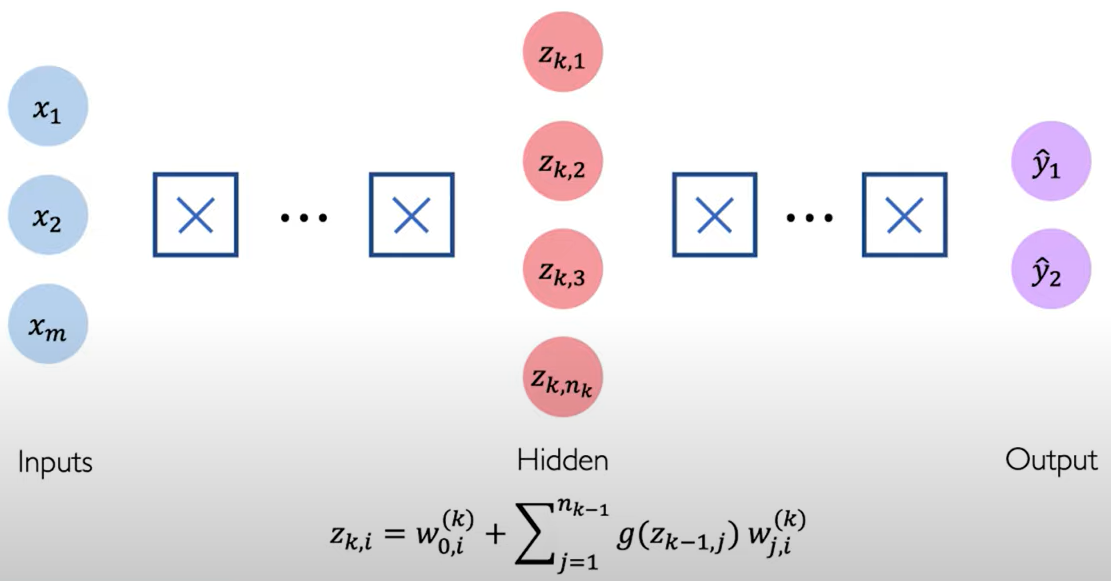
Deep Neural Network.

import tensorflow as tf

model = tf.keras.Sequential([
    tf.keras.layers.Dense(n1),
    tf.keras.layers.Dense(n2),
    :
    tf.keras.layers.Dense(2)
])

Applying Neural Networks

Quantifying Loss. The loss of our network measures the cost incurred from incorrect predictions.

\[\mathcal{L}(f(x^{(i)};\mathbf{W}),y^{(i)})\]

$f(x^{(i)};\mathbf{W})$ is the predicted value, and the $y^{(i)}$ is the actual value.

Empirical Loss. The empirical loss measures the total loss over our entire dataset.

\[\mathbf{J(W)}=\frac{1}{n}\sum_{i=1}^n\mathcal{L}(f(x^{(i)};\mathbf{W}),y^{(i)})\]

$\mathbf{J(W)}$ is the mean of every loss of each individual, and it is also known as: 1) Objective function, 2) Cost function, 3) Empirical risk.

Binary Cross Entropy Loss. Cross entropy loss can be used with models that output a probability between 0 and 1.

\[\mathbf{J(W)}=-\frac{1}{n}\sum_{i=1}^ny^{(i)}\log(f(x^{(i)};\mathbf{W}))+(1-y^{(i)})\log(1-f(x^{(i)};\mathbf{W}))\]

loss = tf.reduce_mean( tf.nn,softmax_cross_entropy_with_logits(y, predicted) )

Mean Squared Error Loss. it can be used with regression models that output continuous real numbers.

\[\mathbf{J(W)}=-\frac{1}{n}\sum_{i=1}^n(y^{(i)}-f(x^{(i)};\mathbf{W}))^2\]

loss = tf.reduce_mean( tf.square(tf.subtract(y, predicted)) )
loss = tf.keras.losses.MSE( y, predicted )

Training Neural Networks

Loss Optimization. We want to find the network weights that achieve the lowest loss:

\[\begin{aligned} W^*&=\underset{W}{\text{argmin}}\frac{1}{n}\sum_{i=1}^n\mathcal{L}(f(x^{(i)};W),y^{(i)})\\&=\underset{W}{\text{argmin}} \mathbf{J(W)} \end{aligned}\]

REMEMBER: Our loss is a function of the network weights.

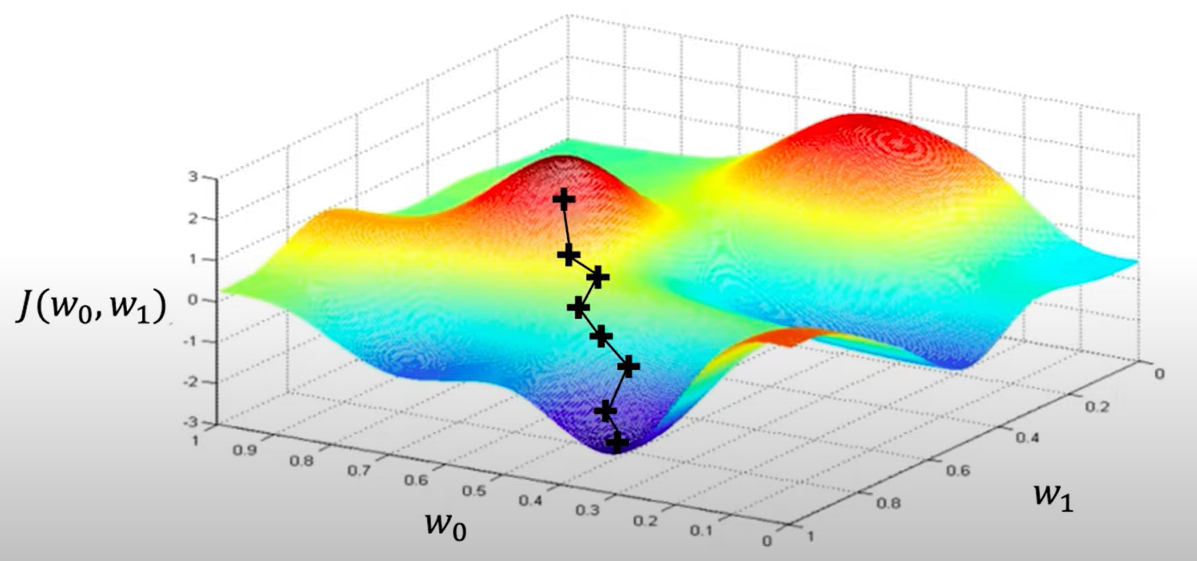
Gradient Descent. Algorithm

1. Initialize weights randomly ~$\mathcal{N}(0,\sigma^2)$
2. Loop until convergence:
   1. Compute gradient, $\frac{\partial J(W)}{\partial W}$
   2. Update weights, $W\leftarrow W-\eta\frac{\partial J(W)}{\partial W}$
3. Return weights

import tensorflow as tf

weights = tf.Variable([tf.random.normal()])

while True:     # loop forever
    with tf.GradientTape() as g:
        loss = compute_loss(weights)
        gradient = g.gradient(loss, weights)

    weights = weights - lr * gradient

We will converge to the local minimum, and we don't know if we converge to the global minimum.

Using Chain Rules repeatedly for every weight in the network using gradients from later layers.

\[\frac{\partial J(W)}{\partial w_1}=\frac{\partial J(W)}{\partial\hat{y}}*\frac{\partial\hat{y}}{\partial z_1}*\frac{\partial z_1}{\partial w_1}\]

Neural Networks in Practice: Optimization

Loss Functions can be difficult to optimize. Remember that Optimization through gradient descent $W\leftarrow W-\eta\frac{\partial J(W)}{\partial W}$, while $\eta$ is the learning rate.

Setting the learning rate.

• Small learning rates converges slowly and gets stuck in false local minima.
• Large learning rates overshoot, become unstable and diverge.
• Stable learning rates converge smoothly and avoid local minima.

How to find the stable learning rates?

1. try lots of different learning rates and see what works "just right".
2. Smarter way! Design an adaptive learning rate that "adapts" to the landscape.

Learning rates are no longer fixed.

• adaptive learning rates can be made larger or smaller depending on:
  • how large gradient is
  • how fast learning is happening
  • size of particular weights
  • etc…

Gradient Descent Algorithms. (and the TF implementation is shown below.)

• SDG
• Adam
• Adadelta
• Adagrad
• RMSProp

tf.keras.optimizers.SDG
tf.keras.optimizers.Adam
tf.keras.optimizers.Adadelta
tf.keras.optimizers.Adagrad
tf.keras.optimizers.RMSProp

---

import tensorflow as tf
model = tf.keras.Sequential([...])

# pick your favorite optimizer
optimizer = tf.keras.optimizer.SGD()

while True: # loop forever

    # forward pass through the network
    prediction = model(x)

    with tf.GradientTape() as tape;
        # compute the loss
        loss = compute_loss(y, prediction)
    
    # update the weights using the gradient
    grads = tape.gradient(loss, model.trainable_variables)
    optimizer.apply_gradients(zip(grads, model.trainable_variables ))

Neural Networks in Practice: Mini-batches

From the Gradient Descent Algorithm, we can know that the $\frac{\partial J(W)}{\partial W}$ can be computationally intensive to compute.

Stochastic Gradient Descent. Algorithm

1. Initialize weights randomly ~$\mathcal{N}(0,\sigma^2)$
2. Loop until convergence:
   1. Pick batch of $B$ data points
   2. Compute gradient, $\frac{\partial J(W)}{\partial W}=\frac{1}{B}\sum_{i=1}^B\frac{\partial J_k(W)}{\partial W}$
   3. Update weights, $W\leftarrow W-\eta\frac{\partial J(W)}{\partial W}$
3. Return weights

It will be fast to compute and a much better estimate of the true gradient.

• Mini-batches is a more accurate estimation of gradient
  • smoother convergence
  • allows for large learning rates
• Mini-batches lead to fast training
  • can parallelize computation (we can split up the batches on separate workers and separate machines)
  • achieve significant speed increases on GPU's

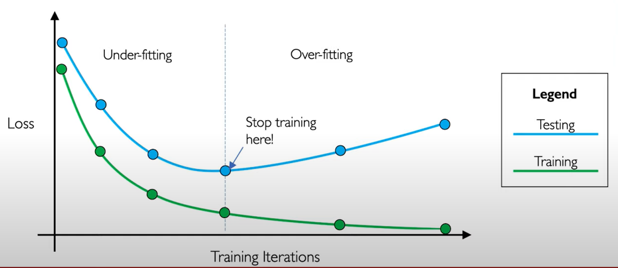
Neural networks in Practice: Overfitting

the problem of overfitting.

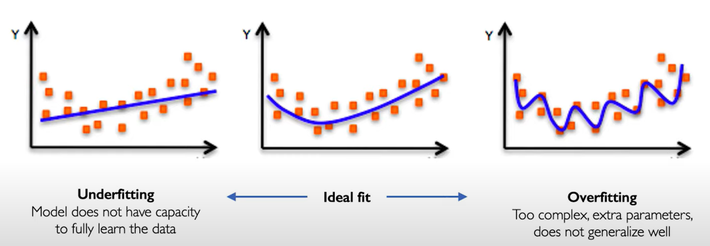
Regularization. it's a technique that constrains our optimization problem to discourage complex models. The goal is to improve the generalization of our model on unseen data. (Specific Regularization methods are shown below.)

1. Dropout. During training, randomly set some activations to zero.
   1. Typically "drop" 50% of activations in layer
   2. Forces network to not rely on any 1 node.
   3. tf.keras.layers.Dropout(p=0.5)
2. Early Stopping. Stop training before we have a chance to overfit.