MIT 6.S191: Recurrent Neural Networks
If you wanna see the original video, click MIT 6.S191: Recurrent Neural Networks.
Deep Learning for Sequence Modeling: Summary
- RNNs are well suited for sequence modeling tasks
- Model sequences via a recurrence relation
- Training RNNs with backpropagation through time
- Gated cells like LSTMs let us model long-term dependencies
- Models for music generation, classification, machine translation, and more.
Lecture 2: Deep Sequence Modeling
Sequence Modeling Applications.
- one to one. binary classification
- many to one. sentiment classification
- one to many. image captioning
- many to many. machine translation
Neurons with Recurrence
The perceptron revisited.
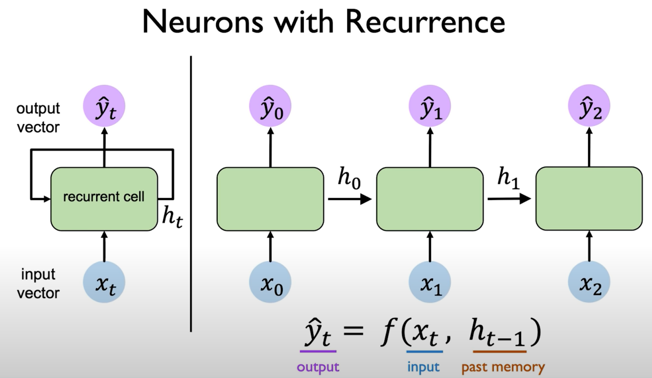
The network's output predictions and its computations are not only a function of the input at a particular time step but also the past memory of cell state denoted by $h$. That is to say, our output depends on both our current inputs as well as the past computations and the past learning that occurred and we can define this relationship via these functions that map inputs to output and these functions are standard neural network operations that alexander introduced in the first lecture.
Our prediction depends not only on the current input at a particular time step, but also on the past memory.
Then, our output is now a function of both the current input and the past memory at a previous time step. This means we can describe these neurons via a recurrence relation which means that we have the cell state that depends on the current input and again on the prior in prior cell states.
The depiction on the right of this line shows these individual time steps being sort of unrolled across time but we could also depict the same relationship by this cycle (this is shown on the loop on the left of the figure which shows this concept of a recurrence).
Recurrent Neural Networks (RNNs)
Apply a recurrence relation at every time step to process a sequence:
\[h_t=f_W(x_t,h_{t-1})\]
- $h_t$ is a cell state;
- $f_W$ is a function with weights $W$;
- $x_t$ is the input;
- $h_{t-1}$ is the old state.
NOTE: the same function and set of parameters are used at every time step in each iteration.
my_rnn = RNN()
hidden_state = [0, 0, 0, 0]

sentence = ["I", "love", "recurrent", "neural"]

for word in sentence:
    prediction, hidden_state = my_rnn(word, hidden_state)

next_word_prediction = prediction
# >>> "networks"
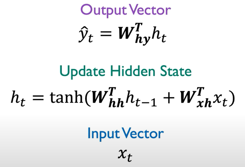
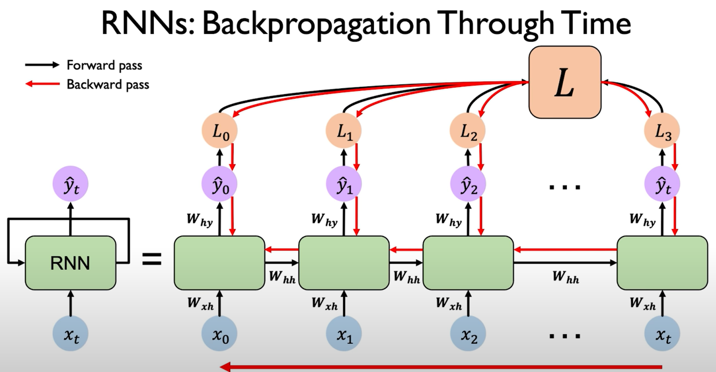
Mathematics behind how the RNN actually update its hidden state and also to produce a predictive output.
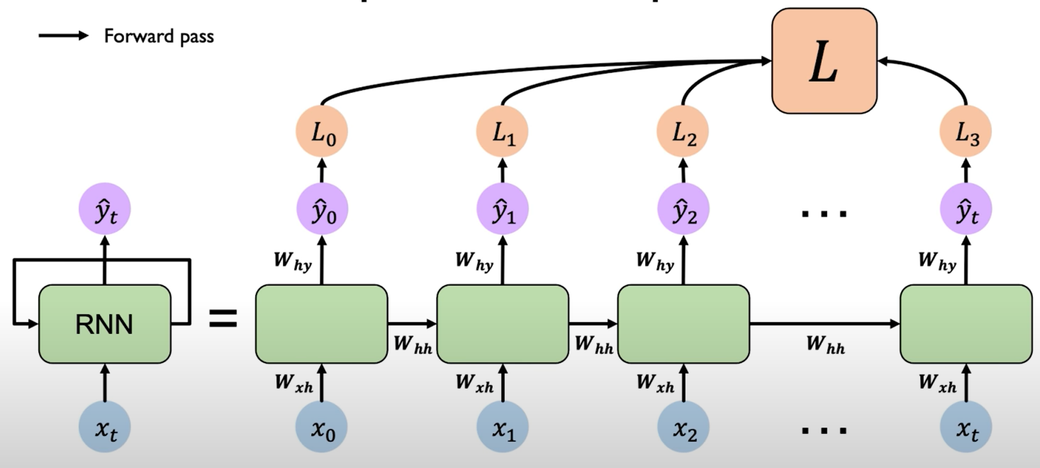
Re-use the same weight matrices at every time step. (L means "Loss" in the figure below)
tf.keras.layers.SimpleRNN(rnn_units)
RNNs Sequence Modeling - Design Criteria. To model sequences, we need to:
- Handle variable-length sequence
- Track long-term dependence
- Maintain information about order
- Share parameters across the sequence
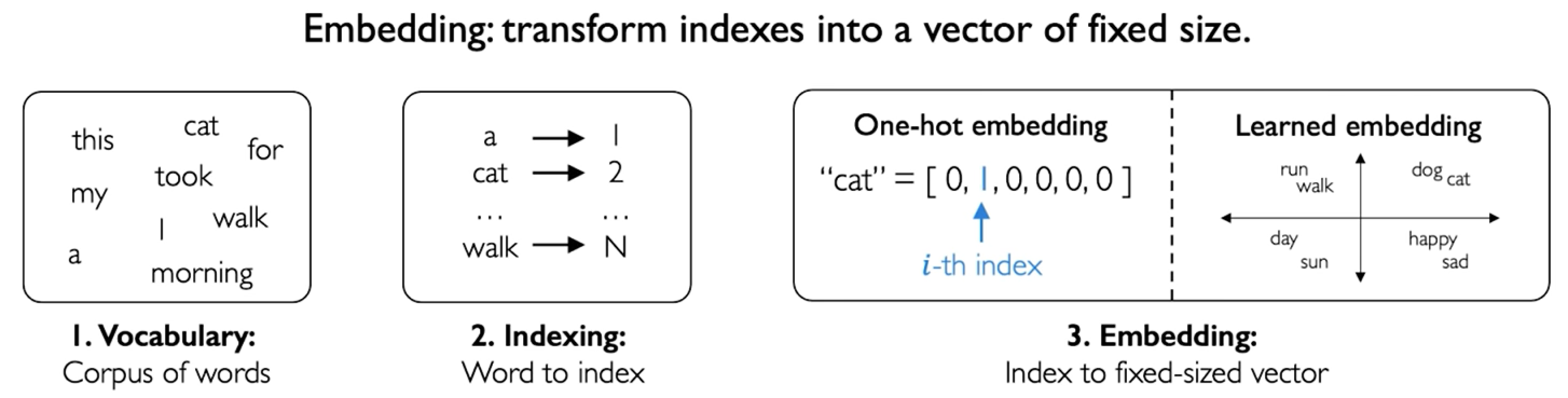
A Sequence Modeling Problem: Predict the Next Word
The first step to tackle this problem: how to represent language to a neural network.
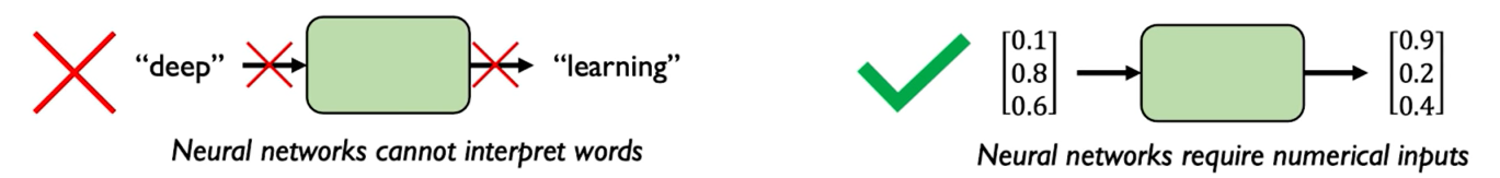
Embedding.
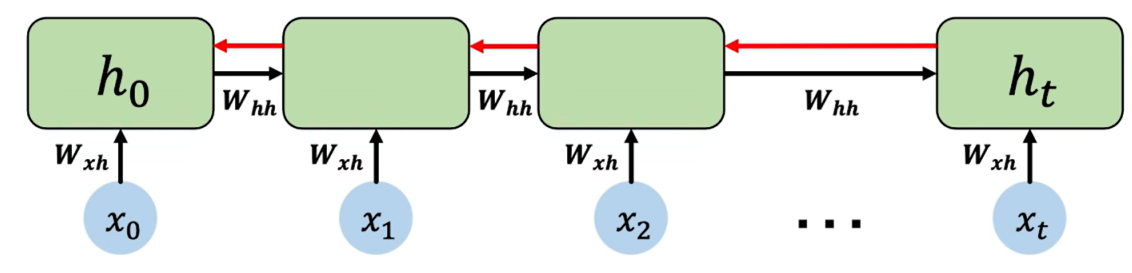
Backpropagation Through Time (BPTT)
Backpropagation algorithm.
- Take the derivative (gradient) of the loss with respect to each parameter;
- Shift parameters in order to minimize loss
Computing the gradient wrt $h_0$ involves many factors of $W_{hh}$ + repeated gradient computation!
with respect to = rwt
- Many values > 1: exploring gradients
- Gradient clipping to scale big gradients
- Many values < 1: vanishing gradients
- Activation function
- Wight initialization
- Network architecture
Why are vanishing gradients a problem? Let's imagine you keeps multiplying a small number something in between 0 and 1 by another small number overtime. That number is going to keep shrinking and shrinking and eventually it's going to vanish. What this means? When this occurs for gradients is that it's going to be harder and harder and harder to propagate errors from our loss function back into the distant past because we have this problem of the gradients becoming smaller and smaller and smaller. Ultimately what this will lead to is we're going to end up biasing the weights and the parameters of our network to capture shorter term dependencies in the data rather than longer dependencies.
In many cases, we have a large gap between what's relevant and the point where we may need to make a prediction. As this gap grows, standard RNNs become increasingly unable to connect the relevant information and that's because of the vanishing gradient problem above.
Trick #1: Activation Function
Using a ReLU function prevents $f'$ from shrinking the gradients when $x>0$.
The derivative of this activation function is greater than one for all instances in which x is greater than zero, and this helps the value of the gradient with respect to our loss function to actually shrink when the values of its inputs are greater than zero.
Trick #2: Parameter Initialization
Initialize weights to identity matrix, and initialize biases to zero.
It can prevent them from shrinking to zero completely.
Trick #3: Gated Cells
Idea: use a more complex recurrent unit with gates to control what information is passed through.
Gated Cells: LSTM, GRU, etc.
Long Short Term Memory (LSTM) networks rely on a gated cell to track information throughout many time steps.
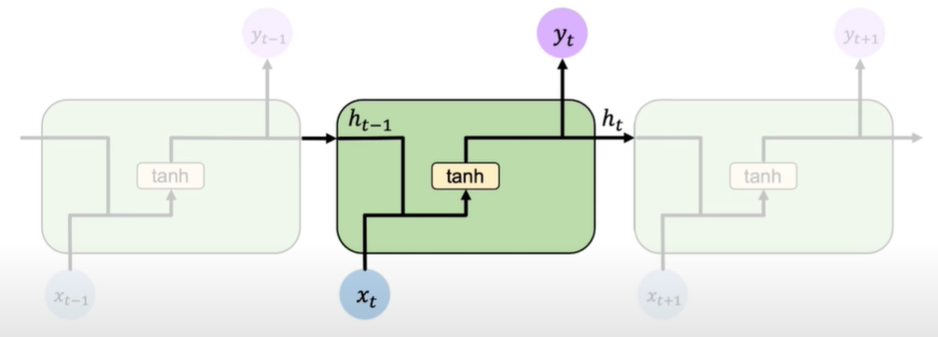
Long Short Term Memory (LSTM) Networks
In a standard RNN, repeating modules contain a simple computation node.
LSTM modules contain computational blocks that control information flow.
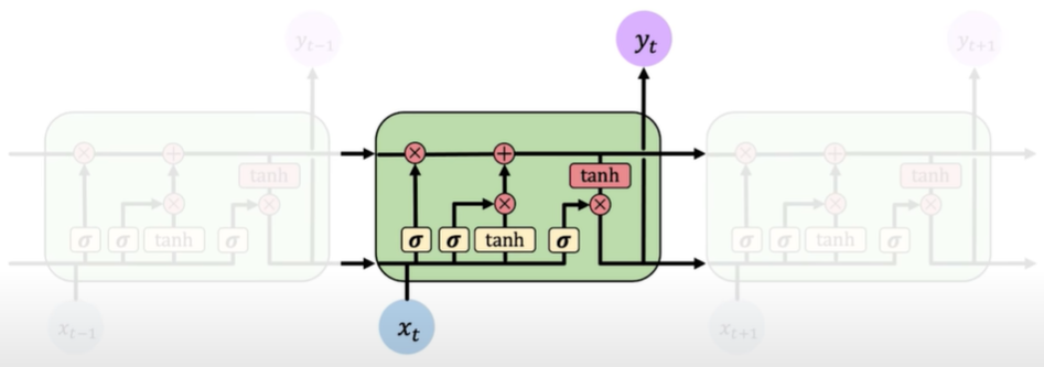
LSTM cells are able to track information throughout many timesteps.
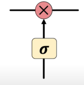
Information is added or removed through structures called gates. Gates optionally let information through, for example via a sigmoid neural net layer and pointwise multiplication.
How do LSTMs work?
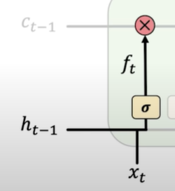
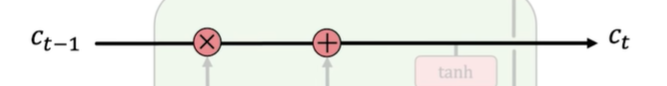
- Forget. LSTMs forget irrelevant parts of the previous state.
- Store. LSTMs store relevant new information into the cell state.
- Update. LSTMs selectively update cell state values.
- Output. The output gate controls what information is sent to the next time step.
1. 2. 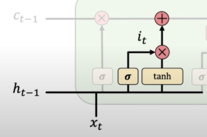
|
3.  4. 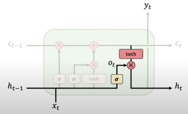
|
Key Concepts of LSTMs:
- Maintain a separate cell state from what is outputted
- Use gates to control the flow of information
- Forget gate gets rid of irrelevant information
- Store relevant information from current input
- Selectively update cell state
- Output gate returns a filtered version of the cell state
- Backpropagation through time with uninterrupted gradient flow
RNN Applications
Example Task: Music Generation.
- Input: sheet music;
- Output: next character in sheet music
Example Task: Sentiment Classification
- Input: sequence of words
- Output: probability of having positive sentiment
loss = tf.nn.softmax_cross_entropy_with_logits(y, predicted)
Example Task: Machine Translation
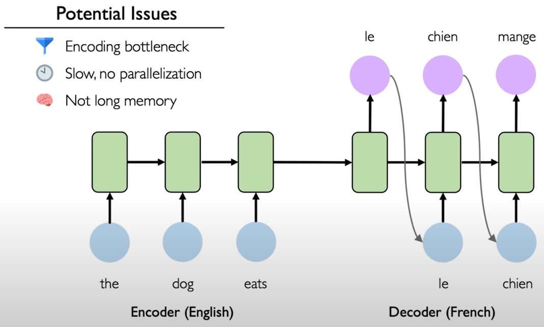
To overcome these potential limitations, a method that't called attention was developed. Instead of the decoder component having access to only the final encoded state that state vector passed from encoder to decoder instead the decoder now has access to the states after each of the time steps in the original sentence and it's weighting of these vectors that is actually learned by the network over the course of training.
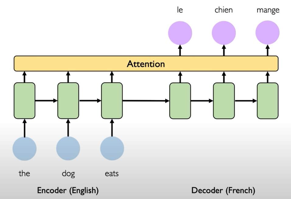
Attention mechanisms in neural networks provide learnable memory access. The system is called attention, because when the network is actually learning the weighting, it's learning to place its attention on different parts of the input sequence to effectively capture a sort of accessible memory across the entirety of the original sequence.
It's a powerful idea and indeed it's the basis of a new class and then rapidly emerging class of models that are extremely powerful for large scale sequential modeling problems and that class of models is called transformers.
A very interesting video on Youtube: MariFlow - Self-Driving Mario Kart w/Recurrent Neural Network