MIT 6.S191: Convolutional Neural Networks
If you wanna see the original video, click MIT 6.S191: Convolutional Neural Networks.
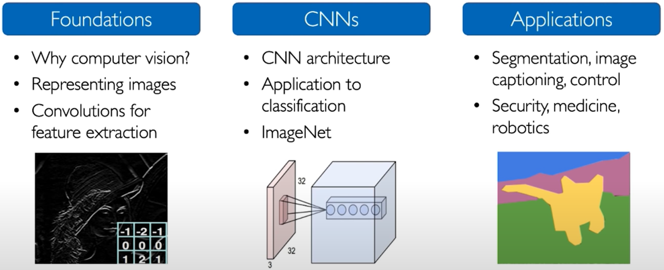
Summary
1. What Computer "See"
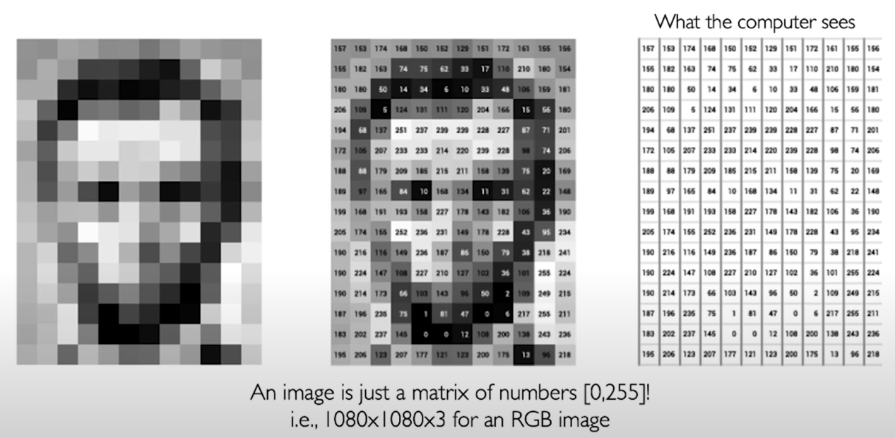
To computers, images are just numbers.
- Regression: output variable takes continuous value
- Classification: output variable takes class label. Can produce probability of belonging to a particular class.
Manual Feature Extraction: Domain knowledge -> Define features -> Detect features to classify.
Learning Feature Representations. Can we learn a hierarchy of features directly from the data instead of hand engineering? (We've mentioned this in the first lecture: MIT Introduction to Deep Learning : 6.S191)
2. Learning Visual Features
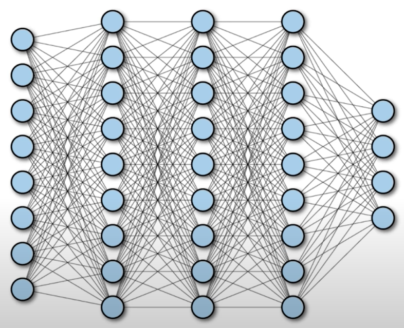
Fully Connected Neural Network (Dense Neural Network).
Input.
- 2D images
- Array of pixel values
Fully Connected Characters:
- Connect neuron in hidden layer to all neurons in input layer
- No spatial information
- And many, many parameters
So, how can we use spatial structure in the input to inform the architecture of the network?
2.1 Using Spatial Structure
IDEA: connect patches of input to neurons in hidden layer. neuron connected to region of input. Only "sees" these values.
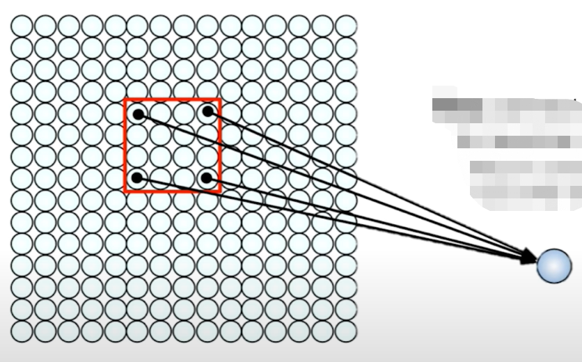
One way we can use the spatial structure would be to actually connect patches of our input. Not the whole input but just patches of the input to neurons in the hidden layer. So before, everything was connected from the input layer to the hidden layer, but now we're just gonna connect only things that are within a single patch to the next neuron in the next layer. Each neuron only sees the values coming from the patch that precedes it.
(patch: a small area of something, especially one that is different from the area around it.)
This will not only reduce the number of weights in our model, but it's also going to allow us to leverage the fact that in an image spatially close pixels are likely to be somewhat related and correlated to each other. That's a fact that we should really take it into account.
Connect patch in input layer to a single neuron in subsequent layer.
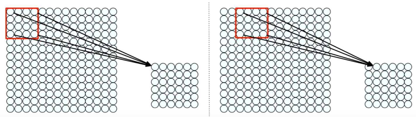
We can basically do this by sliding that patch across the input image. For each time we slide it, we're going to have a new output neuron in the subsequent layer. This way, we can actually take into account some of the spatial structure that inherent to our input, but remember that our ultimate task is not only to preserve spatial structure but to actually learn the visual features. And we do this by weighting the connections between the patches and the neurons.
In practice, there's an operation called a convolution.
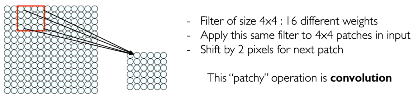
- Apply a set of weights - a filter - to extract local features
- Use multiple filters to extract different features
- Spatially share parameters of each filter
3. Feature Extraction and Convolution - A Case study
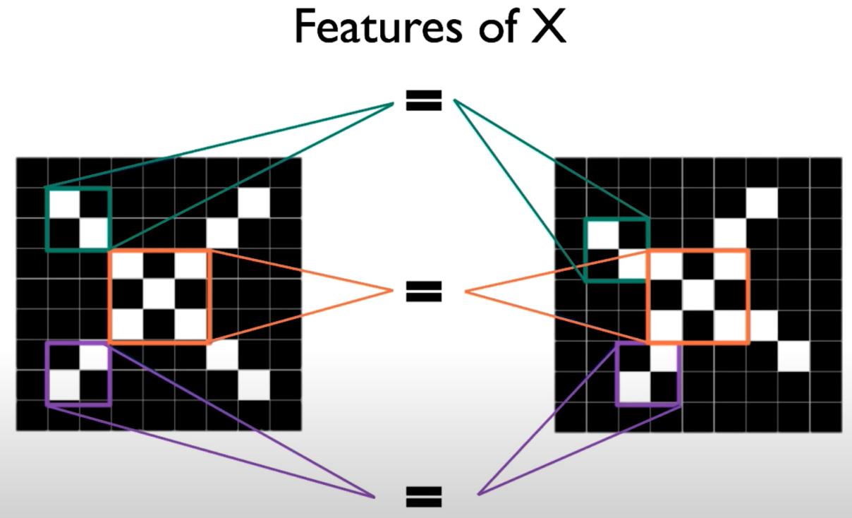
Image is represented as matrix of pixel values and computers are literal! We want to be able to classify an X as an X even if it's shifted, shrunk, rotated, deformed.
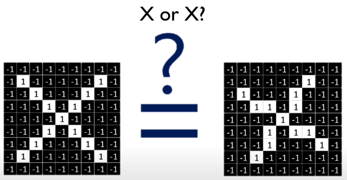
We want our model to basically compare images of a piece of an X (piece by piece) and the really important pieces that it should look for are exactly what we've been calling the features. If our model can find those important (and rough) features that define the X roughly in the same positions, it can get a lot better at understanding the similarity between different examples of X even in the presence of these types of deformities.
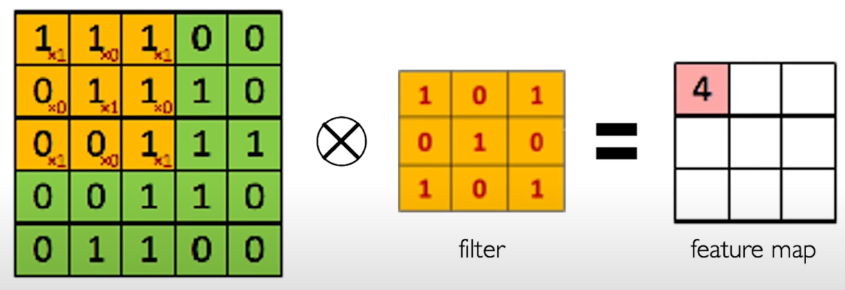
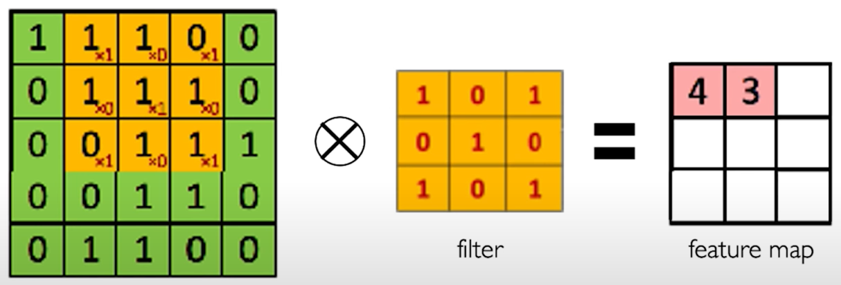
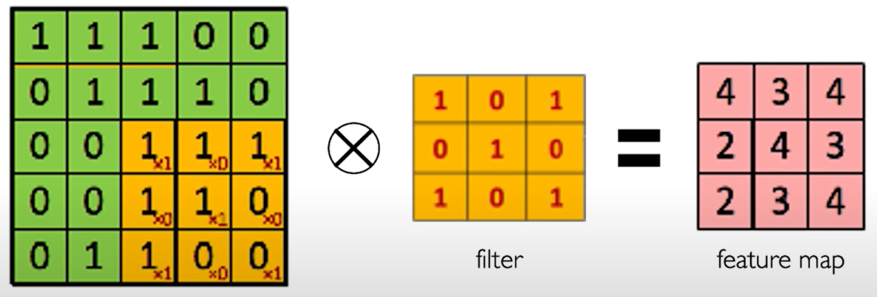
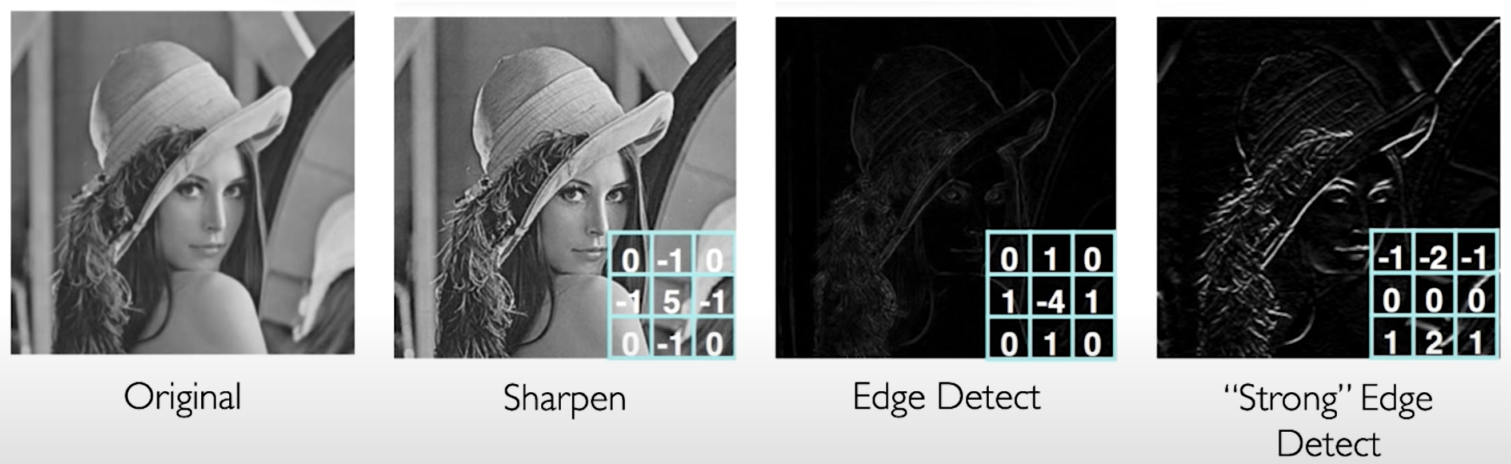
The Convolution Operation. We slide the $3\times 3$ filter over the input image, element-wise multiply, and add the outputs:
|
|
| ... |
|
Producing Feature Maps. Different filter can be used to produce different feature maps.
4. Convolutional Neural Networks (CNNs)
CNNs for Classification.
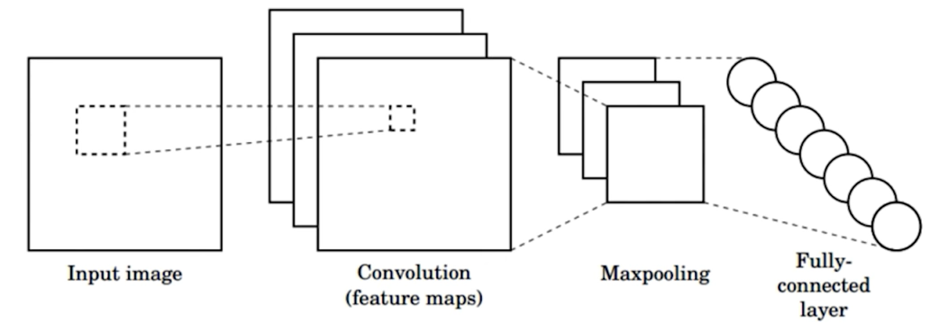
- Convolution: Apply filters to generate feature maps.
- Non-linearity: Often
ReLU. - Pooling: Downsampling operation on each feature map.
tf.keras.layers.Conv2D
tf.keras.activations.*
tf.keras.layers.MaxPool2D
Train model with image data. Learn wights of filters in convolutional layers.
For a neuron in hidden layer:
- take inputs from patch
- compute weighted sum
- apply bias
In the dense layers, we'll need to add on a bias to allow us to shift the activation function, apply and activate it with some non-linearity, so that we can handle non-linear data relationship.
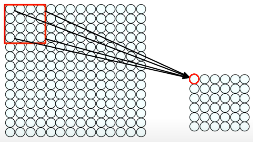
What's special here is that the local connectivity is preserved each neuron in the hidden layer you can see in the right only sees a very specific patch of its inputs. It does not see the entire input neurons like it would have if it was a fully connected layer.
Let's define the actual operation more concretely using a mathematical equation here. We're left with a $4\times 4$ filter matrix, and for each neuron in the hidden layer, its inputs are those neurons in the patch from the previous layer.
\[4\times 4 \text{filter: matrix of weights } w_{ij}\\ \Rightarrow\sum_{i=1}^4\sum_{j=1}^4w_{ij}x_{i+p,j+q}+b\]Summary. 1) applying a window of weights. 2) computing linear combinations. 3) activating with non-linear function.
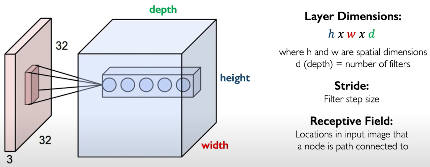
4.1 CNNs: Spatial Arrangement of Output Volume
Previously, we know how to take input image and learn a single feature map. But in reality there are many types of features in our image. How can we use convolutional layers to learn a stack or many different types of features that could be useful for performing our types of task? How can we use this to do multiple feature extraction?
Now the output layer is still convolution but now it has a volume dimension where the height and the width are spatial dimensions dependent upon the dimensions of the input layer.
4.2 Introducing Non-Linearity
- Apply after every convolution operation (i.e., after convolutional layers)
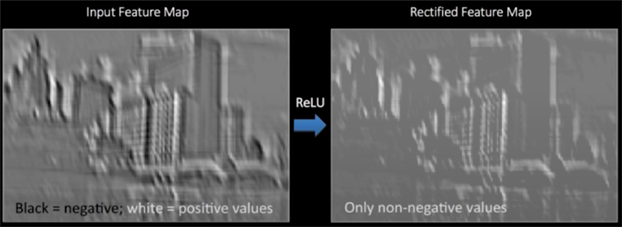
- ReLU: pixel-by-pixel operation that replaces all negative values bt zero. Non-linear operation!
tf.keras.layers.ReLU
4.3 Pooling
Pooling is an operation that is commonly used to reduce the dimentionality of our inputs and of our feature maps while still preserving spatial invariants.
Now, a common technique and a common type of pooling that is commonly used in practice is called Max Pooling.
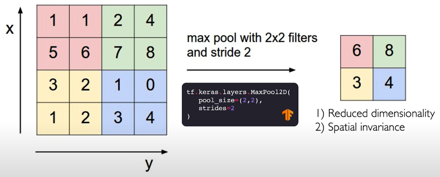
Max Pooling.
- Reduced dimensionality
- Spatial invariance
tf.keras.layers.MaxPool2D(
    pool_size=(2,2),
    strides=2
)
Mean Pooling. Taking the maximum over that patch is one idea. A very common alternative is also taking the average that's called mean pooling.
Taking the average actually represents a very smooth way to perform the pooling operation because you're not just taking a maximum which can be subject to maybe outliers, but you averaging it, so you get a smoother result in your output layer.
| Mean Pooling and Mean Pooling, they both have their advantages and disadvantages. |
4.4 CNNs for Classification: Feature Learning
The CNNs for classification can be broken down into two parts.
4.4.1 Part 1
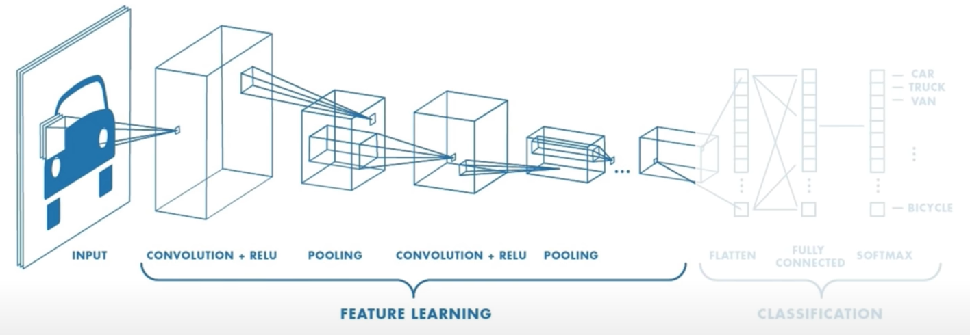
First is the Feature Learning part where we actually try to learn the features in our input image that can be used to perform our specific task. The feature learning part is actually mentioned before in this blog.
Feature Learning:
- Learn features in input image through convolution
- Introduce non-linearity through activation function (real-world data is non-linear!)
- Reduce dimensionality and preserve invariance with pooling
4.4.2 Part 2
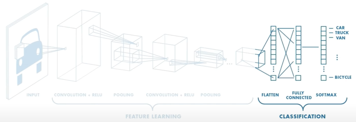
The convolutional layers and pooling provide those the output excuse me of the first part is those high-level features of the input. The second part is actually using these features to perform our classification or whatever our task is in this case. The task is to output the class probabilities that are present in the input image. So we feed those outputted features into a fully connected or dense neural network to perform the classification. We can do this now and don't mind about losing spatial invariance because we've already down sampled our images so much that it's not really even an image anymore, it's actually closer to a vector of numbers, and we can directly apply our dense neural network to that vector of numbers. It's also much lower dimensional now. And We can output a class of probabilities using a function called softmax whose output actually represents a categorical probability distribution.
The spatial invariance of convolution refers to applying the same filter bank F to input patches at all locations.
- CONV and POOL layers output high-level features of input
- Fully connect layer uses these features for classifying input image
- Express output as probability of image belonging to a particular class
import tensorflow as tf

def generate_model():
    model = tf.keras.Sequential([
        # first convolutional layer
        tf.keras.layers.Conv2D(32, filter_size=3, activation='relu'),
        tf.keras.layers.Conv2D(pool_size=2, strides=2),

        # second convolutional layer
        tf.keras.layers.Conv2D(64, filter_size=3, activation='relu'),
        tf.keras.layers.MaxPool2D(pool_size=2, strides=2),

        # fully connected classifier
        tf.keras.layers.Flatten(),
        tf.keras.layers.Conv2D(1024, activation='relu'),
        tf.keras.layers.Conv2D(10, activation='softmax') # 10 output
    ])
    return model
5. An Architecture for Many Applications
What the task is entirely up to you and what you desire. So that's really what makes these networks incredibly powerful.
Task can be
- Classification
- Object detection
- Segmentation
- Probabilistic control
5.1 Object Detection
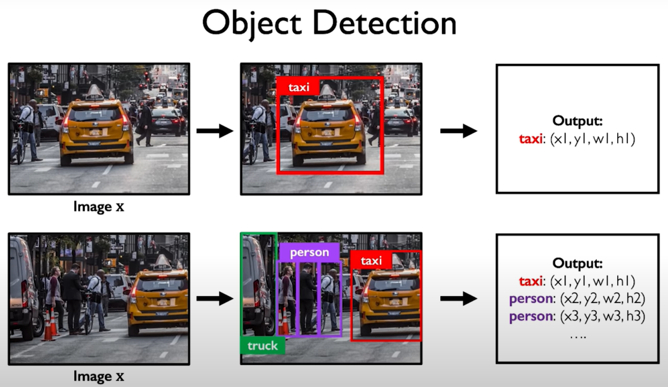
A naive solution. We can start by placing a random box over the input image somewhere. It has some random location, it also has a random size. Then we can take that box and feed it through our normal image classification network. This network's task is to predict what is the class of this image. If there is no class of this box then it simply can ignore it. We repeat this process then we pick another box in the scene and we pass that through network to predict its class and we can keep doing this with different boxes in the scene… In some sense if each of these boxes give us a prediction class we can pick the boxes that do have a class in them and use those as a box where an object is found. Problem: there are way too many inputs, this basically results in boxes and considering a number of boxes that have way too many scales, way to many positions, too many sizes. We can't possibly iterate over our images in all of these dimensions.
5.1.1 Object Detection with R-CNNs
R-CNN algorithm: Find regions that we think have objects. Use CNN to classify.
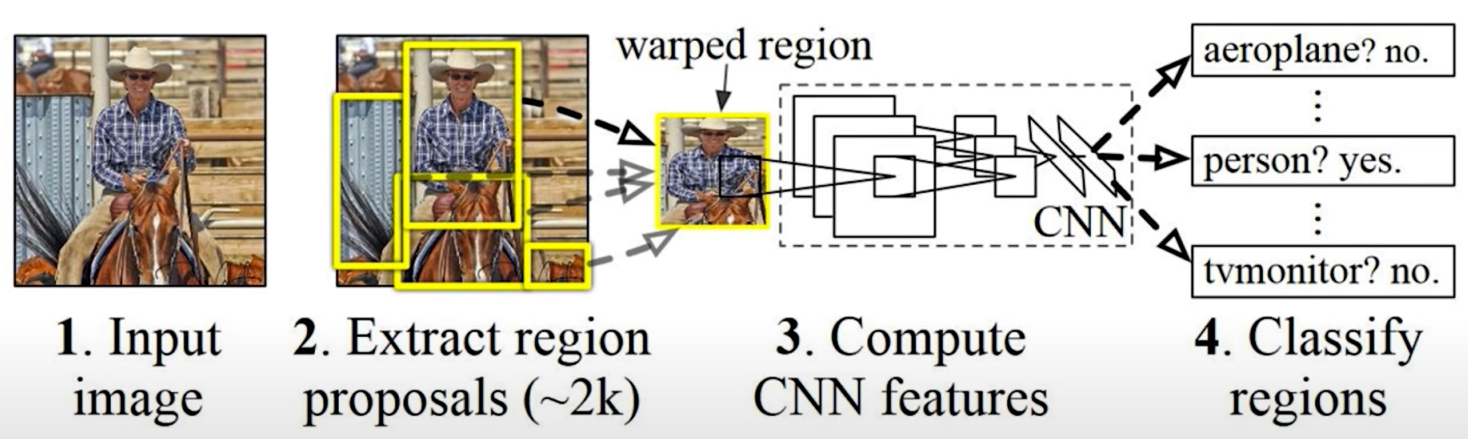
Problems:
- Slow! Many regions; time intensive inference.
- Brittle! Manually define region proposals.
5.1.2 Faster R-CNN Learns Region Proposals
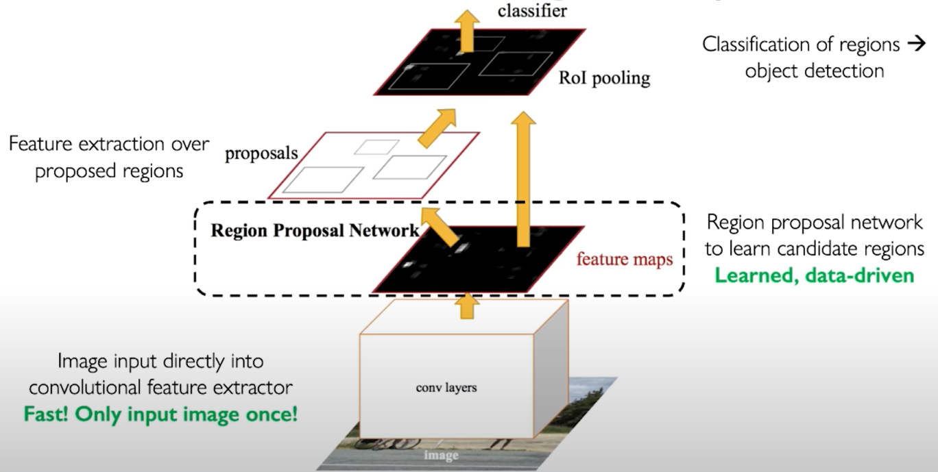
Advantages: It only requires a single forward pass through the model. We only feed in this image once, we have a region proposal network that extracts the regions, and all of these regions are fed on to perform classification on the rest of the image.
5.2 Semantic Segmentation: Fully Convolutional Networks
FCN: Fully Convolutional Network
Network designed with all convolutional layers, with downsampling and upsampling operations.
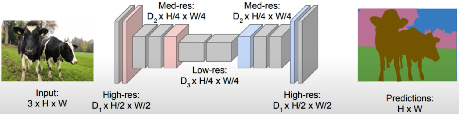
This output is created using an upsampling operation not a downsampling operation. But upsampling allow the convolutional decoder to actually increase its spatial dimension.
tf.keras.layers.Conv2DTranspose
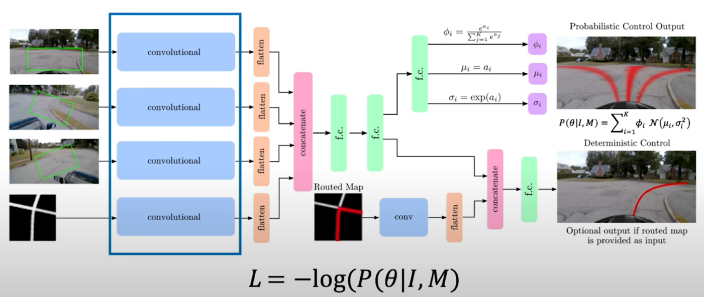
5.3 Continuous Control: navigation from Vision
End-to-End Framework for Autonomous Navigation. Entire model is trained end-to-end without any human labelling or annotations.