FCOS: Fully Convolutional One-Stage Object Detection
The two most important techniques are FPN and correctness. The FPN used in multi-level prediction can ignore the effect of large stride and only needs to select bounding boxes with minimal area to remove intractable ambiguities. Correctness is multiplied with the corresponding classification score to compute the final ranking score, such that those low-mass bounding boxes are filtered out with high probability by the final NMS.
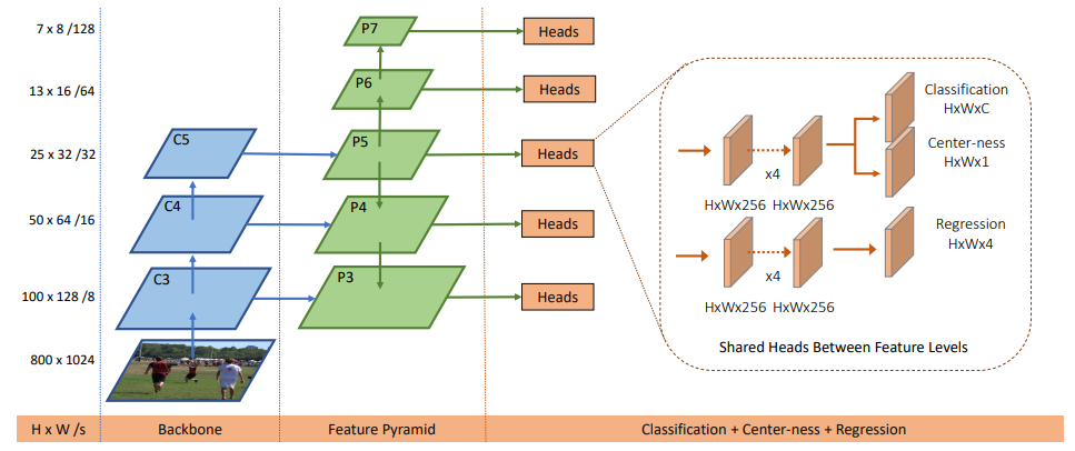
Five levels of feature maps defined as ${P_3,P_4,P_4,P_5,P_6,P_7}$ are used. $P_3\sim P_5$ are produced by the backbone CNNs' feature maps $C_3\sim C_5$ followed by a $1\times 1$ convolutional layer with the top-down connections. $P_6$ and $P_7$ are produced by applying one convolutional layer with the stride being 2 on $P_5$ and $P_6$ respectively. Then the feature levels $P_3,P_4,P_4,P_5,P_6,P_7$ have strides 8,16,32,64 and 128 respectively.
Introduction
Drawbacks of those anchor-based detectors
- Detection performance is sensitive to the sizes, aspect ratios and number of anchor boxes.
- Because of the fixed scales and aspect ratios of anchor boxes, detectors encounter difficulties to deal with object candidates with large shape variations, particularly for small objects.
- The excessive number of negative samples aggravates the imbalance between positive and negative samples in training.
- Anchor boxes also involve complicated computation such as calculating the intersection-over-union (IoU) scores with ground-truth bounding boxes.
FCN-based Framework
These frameworks directly predict a 4D vector plus a class category at each spatial location on a level of feature maps.
These frameworks are similar to the FCNs for semantic segmentation, except that each location is required to regress a 4D continuous vector.
DenseBox are used to crop and resize the training images to a fixed scale.
FPN are applied to tackle the problem of the intractable ambiguity shown below (it is not clear w.r.t. which bounding box to regress for the pixels in the overlapped regions).
A novel "center-ness" branch (only one layer) are utilized to suppress those low-quality detected bounding boxes.
Related work
Anchor-based detector
- In anchor-based detectors, the anchor boxes can be viewed as pre-defined sliding windows or proposals, which can also be seen as training samples.
- Anchor boxes make use of the feature maps of CNNs and avoid repeated feature computation (better than previous detectors like Fast RCNN).
- Excessively many hyper-parameters in anchor-based detector require heuristic tuning, and are specific to detection tasks (deviate from a neat fully convolutional network architectures used in other dense prediction tasks such as semantic segmentation.)
Anchor-free detector
- YOLOv1 is a popular anchor-free detector. YOLOv1 predicts bounding boxes at points near the center of objects. Only the points near the center are used since they are considered to be able to produce higher quality detection. But the YOLOv1 suffers from low recall, which is also the reason why anchor-based detector are proposed.
- FCOS takes advantages of all points in a ground truth bounding box to predict the bounding boxes and the low-quality detected bounding boxes are suppressed by the proposed “center-ness” branch. (recall is comparable to those anchor-based detectors.)
- CornerNet is an one-stage anchor-free detector, which detects a pair of corners of a bounding box and groups them to form the final detected bounding box. It requires much more complicated postprocessing to group the pairs of corners belonging to the same instance.
- Another family of anchor-free detectors are based on DenseBox. The family of detectors have been considered unsuitable for generic object detection due to difficulty in handling overlapping bounding boxes and the recall being relatively low.
Approach
FCOS: Fully convolutional one-stage object detector
- $F_i\in\mathbb{R}^{H\times W\times C}$: the feature maps at layer $i$ of a backbone CNN
- $s$: the total stride until the layer
- ${B_i}$: the ground-truth bounding boxes for an input image.
- $B_i=(x_0^{(i)},y_0^{(i)},x_1^{(i)},y_1^{(i)},c^{(i)})\in\mathbb{R}^4\times{1,2,…,C}$
- $(x_0^{(i)},y_0^{(i)})$ and $(x_1^{(i)},y_1^{(i)})$ denote the coordinates of the left-top and right-bottom corners of the bounding boxes.
- $c^{(i)}$ is the class that the object in the bounding box belongs to.
- $C$ is the number of classes.
For each location $(x,y)$ on the feature map $F_i$, it can be mapped onto the input images as $(\left\lfloor\frac{s}{2}\right\rfloor+xs,\left\lfloor\frac{s}{2}\right\rfloor+ys)$, which is near the center of the receptive filed of the location $(x,y)$.
In other words, our detector directly views locations as training samples instead of anchor boxes in anchor-based detectors, which is the same as FCNs for semantic segmentation.
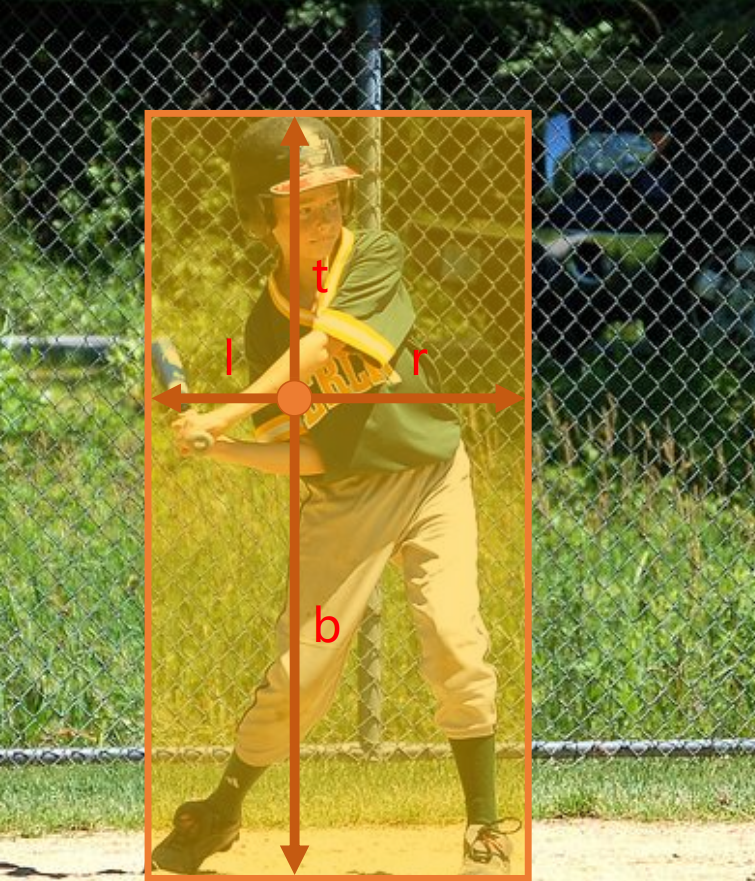
Formally, if location $(x, y)$ is associated to a bounding box $B_i$, the training regression targets for the location can be formulated as
\[\begin{matrix} l^\ast=x-x_0^{(i)},&t^\ast=y-y_0^{(i)},\\ r^\ast=x_1^{(i)}-x,&b^\ast=y_1^{(i)}-y. \end{matrix}\tag{1}\][Possible reason for FCOS outperforming its anchor-based counterparts] It is worth noting that FCOS can leverage as many foreground samples as possible to train the regressor. It is different from anchor-based detectors, which only consider the anchor boxes with a highly enough IOU with ground-truth boxes as positive samples.
Network outputs
Instead of a multi-class classifier, C binary classifiers are trained.
Loss function
\[\begin{aligned} L\left(\left\{\boldsymbol{p}_{x, y}\right\},\left\{\boldsymbol{t}_{x, y}\right\}\right) &=\frac{1}{N_{\text {pos }}} \sum_{x, y} L_{\mathrm{cls}}\left(\boldsymbol{p}_{x, y}, c_{x, y}^{*}\right) \\ &+\frac{\lambda}{N_{\operatorname{pos}}} \sum_{x, y} \mathbb{1}_{\left\{c_{x, y}^{*}>0\right\}} L_{\mathrm{reg}}\left(\boldsymbol{t}_{x, y}, \boldsymbol{t}_{x, y}^{*}\right), \end{aligned}\tag{2}\]- $L_{cls}$: the focal loss
- $L_{reg}$: the IOU loss
- $N_{pos}$: the number of positive samples
- $\lambda$ being 1 in this paper is the balance weight for $L_{reg}$
- $\mathbb{1}{\left{c{x, y}^{*}>0\right}}$: the indicator function
Inference
Given an input images, we forward it through the network and obtain the classification scores $p_{x,y}$ and the regression prediction $t_{x,y}$ for each location on the feature maps $F_i$.
The location with $p_{x,y}>0.05$ as positive samples and invert Eq.(1) to obtain the predicted bounding boxes.
Multi-level prediction with FPN for FCOS
Two possible issues
Low BPR caused by large stride
The large stride (e.g., 16$\times$) of the final feature maps in a CNN can result in a relatively low best possible recall (BPR).
For anchor based detectors, low recall rates due to the large stride can be compensated to some extent by lowering the required IOU scores for positive anchor boxes.
For FCOS, at the first glance, one may think that the BPR can be much lower than anchor-based detectors because it is impossible to recall an object which no location on the final feature maps encodes due to the a large stride.
But the BPR is actually not a problem of FCOS, and the BPR can be improved further to match the best BPR (the anchor-based RetinaNet can achieve) with multi-level FPN prediction.
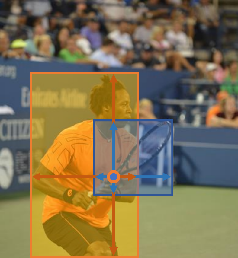
Intractable ambiguity
Following FPN, different sizes of objects are detected on different levels of feature maps.
Unlike anchor-based detectors, which assign anchor boxes with different sizes to different feature levels.
In FCOS, we directly limit the range of bounding box regression for each level (2 steps):
Step 1. Regression targets $l^\ast,t^\ast,r^\ast,b^\ast$ for each location on all feature levels.
Step 2. If a location satisfies $\max(l^\ast,t^\ast,r^\ast,b^\ast)>m_i$ or $\max(l^\ast,t^\ast,r^\ast,b^\ast)<m_{i-1}$, it is set as a negative sample. (not require to regress a bounding box; $m_i$ is the maximum distance that feature level $i$ need to regress) In this work, $m2,…,m7=0,64,128,256,512,\infty$.
Since objects with different sizes are assigned to different feature levels and most overlapping happens between objects with considerably different sizes. If a location, even with multi-level prediction used, is still assigned to more than one ground-truth boxes, we simply choose the ground-truth box with minimal area as its target.
Different feature levels are required to regress different size range, instead of using the standard $\exp(x)$, we make use of $\exp(s_ix)$ with a trainable scalar $s_i$ to automatically adjust the base of the exponential function for feature level $P_i$.
Center-ness for FCOS
Due to a lot of low-quality predicted bounding boxes produced by location far away from the center of an object, we defined the center-ness target as
\[\text { centerness }^{*}=\sqrt{\frac{\min \left(l^{*}, r^{*}\right)}{\max \left(l^{*}, r^{*}\right)} \times \frac{\min \left(t^{*}, b^{*}\right)}{\max \left(t^{*}, b^{*}\right)}}\]The loss is added to the loss function Eq. (2). When testing, the final score (used for ranking the detected bounding boxes) is computed by multiplying the predicted center-ness with the corresponding classification score.
Thus the center-ness can down-weight the scores of bounding boxes far from the center of an object. As a result, with high probability, these low-quality bounding boxes might be filtered out by the final non-maximum suppression (NMS) process, improving the detection performance remarkably.
NMS is introduced HERE with intuitive graphical representations.
Extra Knowledge: What is an ablation study?
The original meaning of “Ablation” is the surgical removal of body tissue. The term “Ablation study” has its roots in the field of experimental neuropsychology of the 1960s and 1970s, where parts of animals’ brains were removed to study the effect that this had on their behaviour.
In the context of machine learning, and especially complex deep neural networks, “ablation study” has been adopted to describe a procedure where certain parts of the network are removed, in order to gain a better understanding of the network’s behaviour.
References
- Tian, Z., Shen, C., Chen, H., & He, T. (2019). Fcos: Fully convolutional one-stage object detection. In Proceedings of the IEEE/CVF international conference on computer vision (pp. 9627-9636).
- https://stats.stackexchange.com/questions/380040/what-is-an-ablation-study-and-is-there-a-systematic-way-to-perform-it/380233#380233
- Lin, T. Y., Dollár, P., Girshick, R., He, K., Hariharan, B., & Belongie, S. (2017). Feature pyramid networks for object detection. In Proceedings of the IEEE conference on computer vision and pattern recognition (pp. 2117-2125).